
The Vol-Control Playbook - A Macro Manv & MacroTourist Deep Dive
How a Nokia Phone, a Pint, and some Python built a Market Flow Model


An exciting part of finance, is the people you meet. A few weeks ago in London, I missed the official MacroTourist meetup. So naturally, I did the only sensible thing: bent my schedule and managed to squeeze in a cheeky pint with Kevin before he rushed off to his next meeting.
The conversation got off to a curious start when I pulled out an old-style Nokia phone. It’s part of my (likely futile) attempt to curb my screen time. Nevertheless, that odd choice sparked a great conversation about habits, heuristics, volatility, and everything in between. Kevin, I found, is just as curious and thoughtful in person as he is on the page.
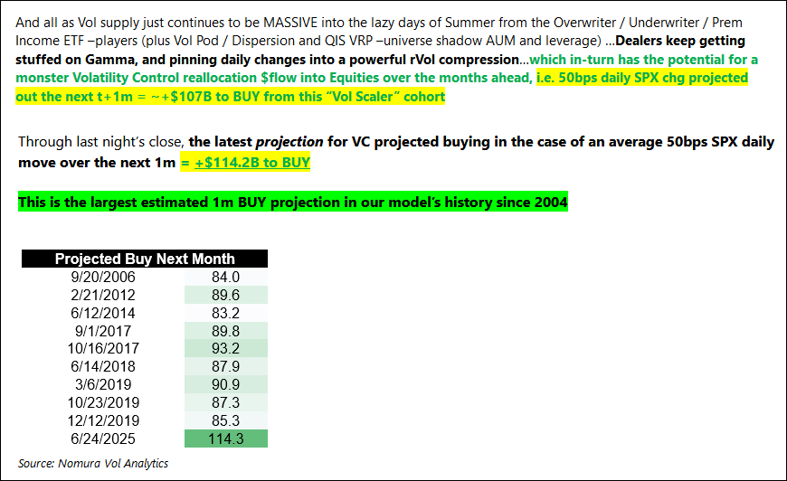
A few days later, I got a message from Kevin. He was on a flight, chewing over the summer flow setup as many wall street strategists were highlighting how this summer would experience the largest amount of buying ever recorded from vol-control funds (see below). He had a sharp insight: the precise timing of those flows might be the single biggest driver of a slow summer market.
The idea? Build a model to forecast forward flows based on assumed volatility paths. We spent the next week building it out, and here’s what we found:
(The below draws largely from Kevin’s original write-up, shared here as part of our collaboration).
Vol-control strategy obsession?
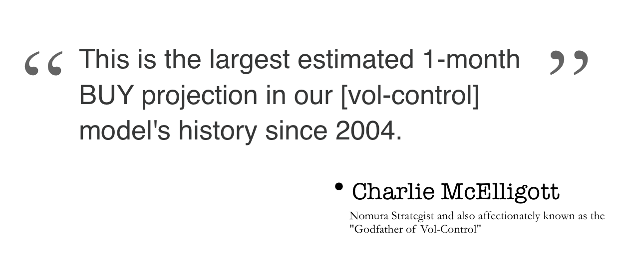
Although lots of strategists are highlighting the increasing effect that vol-control strategies are having on the marketplace, we can all probably agree that the “Godfather of Vol-Control” is Nomura’s Charlie McElligott. He’s been writing about this strategy long before it was cool. Therefore, when Charlie warns how this is the largest 1-month BUY projection in history, it behooves us to pay attention.
For those unfamiliar with vol-control strategies, see Kevin’s brilliant original piece from a couple of years ago Explaining Vol Control Funds, from which I have summarised the basic concept below:
Vol-control funds adjust equity exposure to maintain a target volatility level—buying more when markets are calm and selling when volatility rises. Unlike option-driven flows (like vanna/charm), these funds react to realized volatility, not implied. They use exponential smoothing of short- and long-term volatility measures to de-lever quickly but re-risk slowly, creating pro-cyclical market feedback. Popular among insurance and pension funds for capital efficiency, they can amplify both rallies and selloffs depending on market conditions. Understanding their mechanics helps explain otherwise puzzling market strength or weakness.
Originally, the vol-control bid was expected to be nearly exhausted. However, the analysis below suggests it may persist through the rest of the summer. Let’s unpack how the strategy actually behaves.
Understanding the strategy’s behaviour
At first glance, the S&P 500 vol-control strategy seems simple enough. Calculate the 30 and 90-day historical volatility, take the higher of the two series as the “realized volatility”, apply some math to calculate the desired exposure for a given target volatility, and then rebalance accordingly. However, there is an added twist. The 30 and 90-day historical volatility are smoothed using an exponential weighting function that assigns more weight to nearer observations. As an added kink, the exponential rate at which they decay differs.
Therefore, our first step was to create the “Corrected 30-day and 90-day Volatility” (this is the volatility that is smoothed according to S&P 500 vol-control strategy inputs):

The blue line is the “corrected 30-day volatility” while the orange is the “corrected 90-day volatility.” These are the historical volatilities with the appropriate exponential smoothing function applied.
To forecast future flows, we need to make an assumption of “forward volatility.” Think about this as our best guess about the level of volatility in the next few months. For this model, we’ve used 12% (the approximate level of volatility we’ve experienced over the last month). Plugging that estimate into the model, we can forecast the “corrected 30-day volatility” (denoted by the red line) and the “corrected 90-day volatility” (expressed as the green line).
Once we have both the historical and forward 30 and 90-day corrected volatilities, we can create the series based on the maximum of the two values.

I has added some items like the top spikes for 30 and 90-day volatilities, and the point where that spike mostly “rolls off” the calculation.
Once we have this series, we can create an estimate about future flows. Now, a word of warning; no one truly knows how much is indexed to these strategies. There are no ETFs benched to these indexes. These vol-control strategies are more popular with institutional longer-term portfolio managers. And the other big user is the structured note community. Therefore, any sort of approximation of capital following these strategies is just a guess. There was a Reuters article from a few years back that quoted Deutsche Bank’s estimate of $250 billion. However, reverse engineering Nomura’s Charlie McElligott’s flows results in a number a few multiples of that estimate.
I have no idea of the actual number, but I don’t think it matters. We can see the effect in the marketplace from this strategy, so we know it’s important. I’d rather focus on the timing of the flows as opposed to debating the size. For this exercise, I’ve chosen a number larger than DB’s estimate, but lower than Charlie’s implied level.
These flows are also sensitive to the target volatility. If the client is indexed to a 15% target vol index, they will de- and re-lever more quickly than someone indexed to 5% target vol. After I wrote my original piece, I had a structured note trader reach out and tell me that most of the notes are struck against a low target vol. He mentioned that 5% was the most popular choice. However, I suspect that the pension funds and endowments that are using this strategy are likely higher. A 10% or 12% target vol seems more appropriate for this crew.
It’s a complete arbitrary decision, but I have created some charts using $500 billion indexed to a 7% target volatility with a forward volatility of 12%.
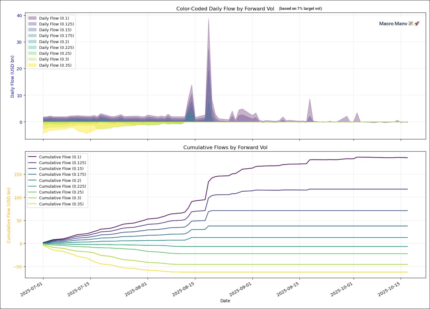
Let’s start with the projected flows over the next month:

What immediately jumps out is the huge buying spike in the middle of August.
What’s causing that?
It’s the rolling off of the Liberation Day tariffs volatility. Recall back to our “Corrected volatility” chart, but this time with an added series of the “AUM in Equities” which we can approximate as a delta for the strategy:

Now, let’s remember that this is based on forward volatility of 12%. That assumes the market will stay subdued and quiet.
But one of the great things about the model is that we can see what happens at different forward volatilities. For example, here is a chart of cumulative flows based on 35%, 30%, 25%, 22.5%, 20%, 17.5%, 15%, 12.5% and 10% forward vols:
Here’s another way to look at it. Kevin created a table of individual daily flows based on those different forward volatilities.
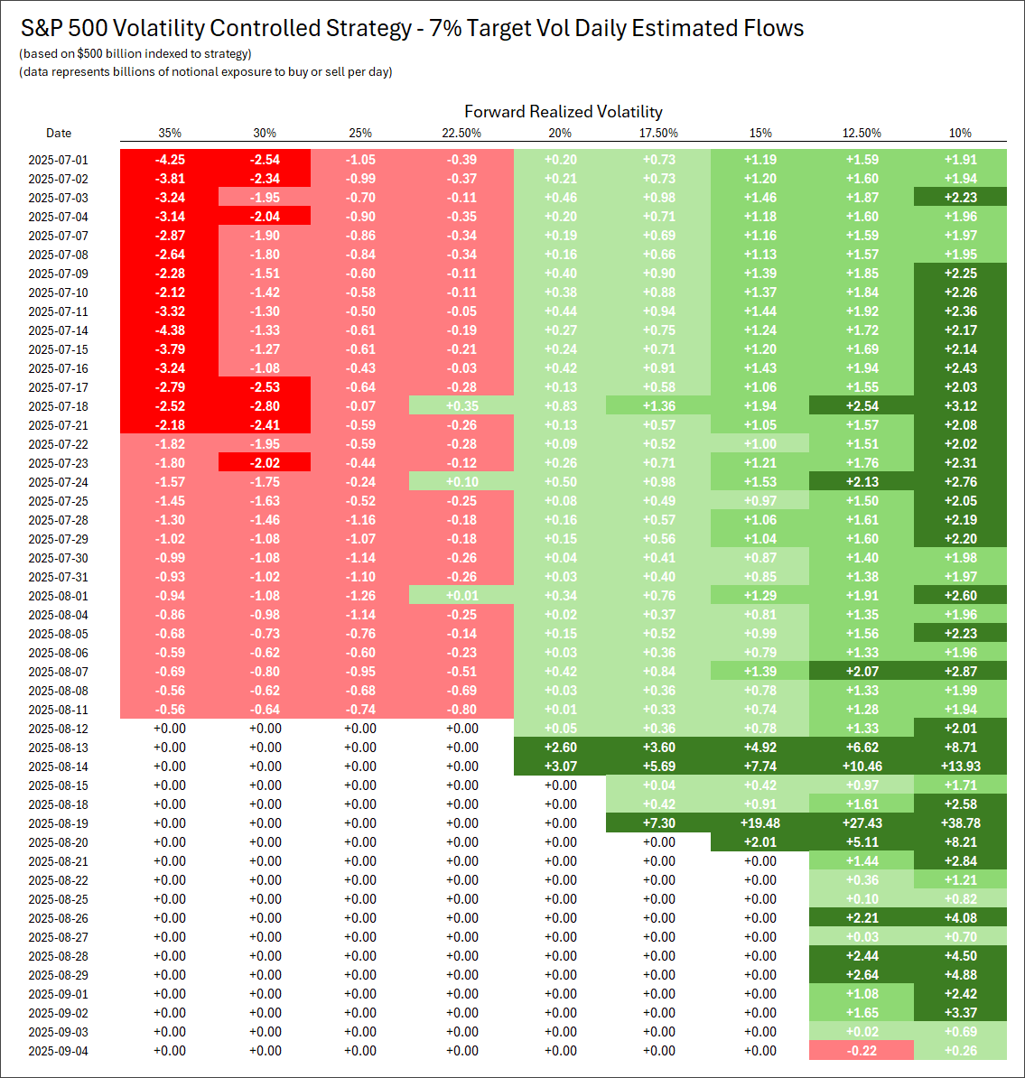
This chart highlights the most important insight about vol-control and its effect on the market. Right now, the “corrected volatility” is running somewhere between 20% and 22.5%. Realized volatility is running down at around 12%, so the vol-control strategies are buying stock aggressively. This will continue until the vol-control strategies “catch up” with current volatility. Remember, these strategies are quick to de-lever, but then take their time buying it back.
Even at 15% realized volatility, there will be a consistent bid from these strategies in the market for some time to come. Even the 7% target vol strategy won’t get fully invested for a 15% equilibrium volatility until August 20th.
When strategists like Charlie McElligott forecast the largest positive flow in the history of this strategy over the next month, it is all based on realized volatility continuing to be subdued. And that’s the important thing to realize about vol-control — it’s reflexive. If vol-control funds keep buying all summer, it will likely keep volatility capped, which will increase the amount of their buying. This will continue until approximately mid-August when they will finally become fully invested based on volatility.
My initial belief was that this state would be reached more quickly. I didn’t expect it to take another month and a half. Yet, that’s what the model is showing. This is why taking the time to forecast the index is so valuable.
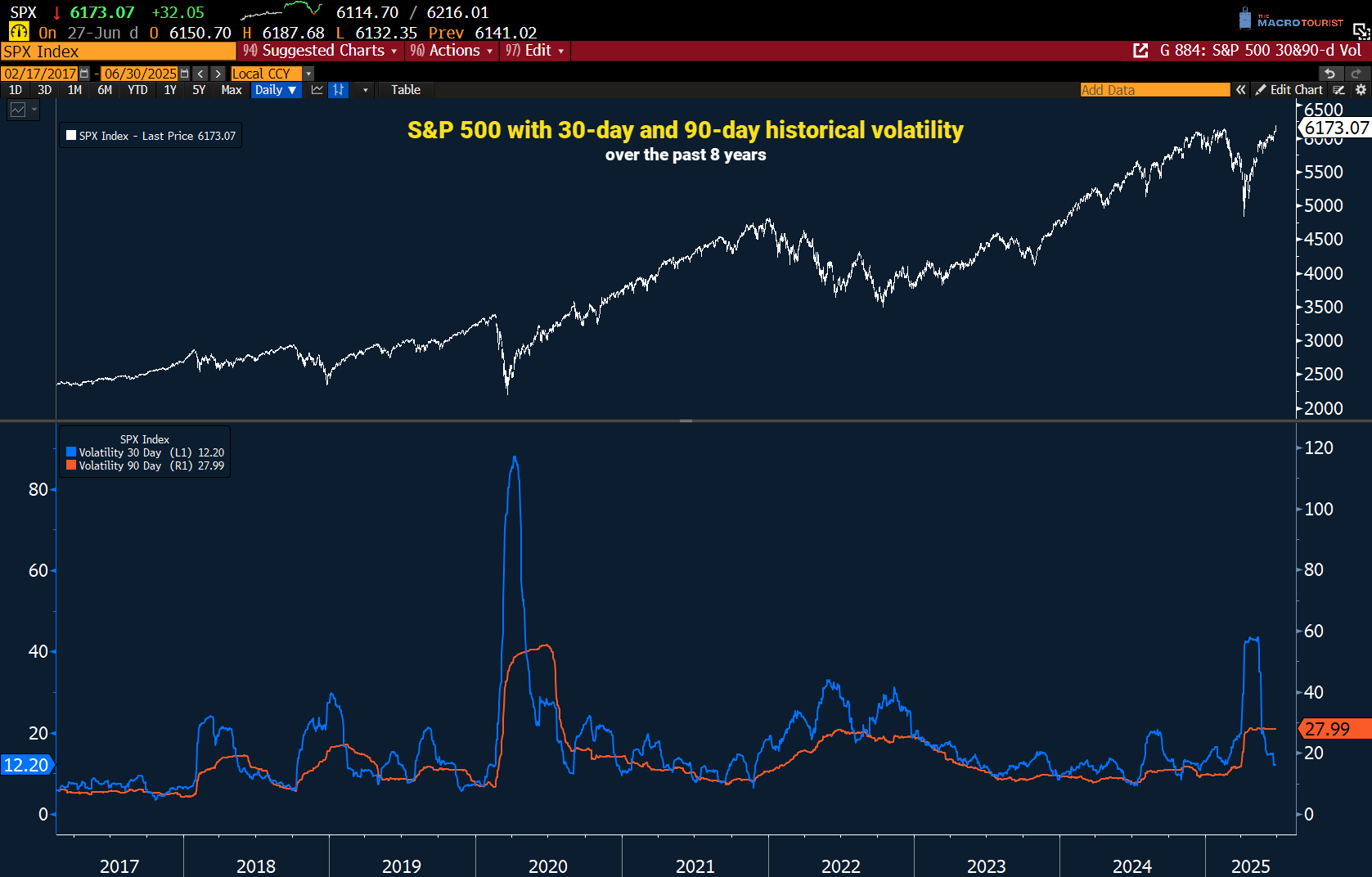
However, it’s also extremely important to understand that this buying can dry up relatively quickly if the market were to become volatile. The S&P 500 realized a 30-day volatility of more than 20% for most of 2022.
If the economy were to roll over and cause some selling in the stock market, volatility would likely spike. If it were to rise high enough, these volatility control funds would go from a buyer to a seller quickly.
I am not predicting that outcome. Absent a fundamental change, realized volatility will likely stay low enough to cause vol-control funds to be bid all summer long. Therefore, in a quiet market, the most likely outcome is a consistent grind higher. This is exactly what we’ve seen for the past week. I don’t think that’s a coincidence. Although I hate this conclusion, it’s still not time to get short. There is an old Wall Street adage, “never short a dull market.” We should probably change that to, “never short a quiet summer market when the vol-control funds are still in the process of re-levering.”
Thank you all for reading and, thanks again to Kevin for the collaboration — and for reminding me why this work is so much fun.
Good luck out there!.
Macro Manv
P.S. For the finance geeks: as previously mentioned, here is a link to the code. I have included a python version that runs with yFinace (Yahoo Finance) and another that works with BQNT.

Inputs are all editable at the top of the notebook so that you can incorporate your own forward volatility forecast and understand how vol-control funds will react. The BQNT version has an interactive chart where you can dial different assumptions. If you find it useful, please reach out and let me know!
Brilliant!